


How AI Beats Doctors in Brain Tumor Detection: The Power of CNNs

When a radiologist classifies a brain tumor, it depends solely on their abilities and experience. And the cost for misclassifying a brain tumor is exceptionally high, often drastically reducing patient survivability. This is not an area where doctors can afford to make a mistake, yet they so often do. According to JHU medicine, there are more than 120 different types of brain tumors, lesions and cysts. There are significant brain tumor size, shape, and intensity variations for the same tumor type, which leads to difficulty with manual diagnosis. Accurate classification is important because different types of brain tumors respond differently to treatment. So, can Artificial Intelligence really make a difference?
Your first thought might be heightened skepticism, which I would wholly understand. How can a computer tell the difference between Tumor X and Tumor Y, when that question has stumped even our most adept clinicians? The answer lies in Convolutional Neural Networks.
What are Convolutional Neural Networks(CNNs)?
A CNN is a deep learning model that can automatically learn to recognize patterns in images. Every image in a digital device is stored as a matrix of pixel values. Each pixel in the image is composed of 3 values(RGB), allowing the screen to display a wide range of colors by combining different intensities of red, green, and blue. If we took an image of a koala for example, it would have a pixel size of 1920 x 1080 x 3.

A CNN is made up of many convolutional layers, pooling layers, and a fully-connected layer. In the convolutional layer, a CNN utilizes a filter, also known as a kernel, to apply a convolution operation across an image. A filter is a 3x3 matrix that is made to detect a certain pattern in an image, for example an eye in the Koala above. The filter moves across the image taking the dot product of the 2 matrices and saving the values to a feature map. Wherever you see a 1 or a number close to 1 on the feature map it means a Koala’s eye was detected. The way CNNs work is through location invariant feature detection. This means if we were to use a different picture of a koala, where the koala is hanging upside down and the eye is located near the bottom of the image, the filter would still be able to detect it.

For a koala, we’d of course need more filters, so the first Convolutional layer might also have filters for the ears and nose. Each of these filters would form their own feature map after running the convolution operation on the input image. The beauty of CNNs is that previously generated feature maps and their detected simple features are used to build more complex ones in later convolutional layers. So the filter maps for the eyes/ears/nose would be used to create a 3d filter map for the head of the koala. The first slice would represent the eyes, the second slice representing the ears, and the third slice representing the nose. In theory, the first filter applied to the image wouldn’t be something recognizable like an eye. It would be a straight line or an edge and slowly build up through each convolutional layer to recognize an eye.

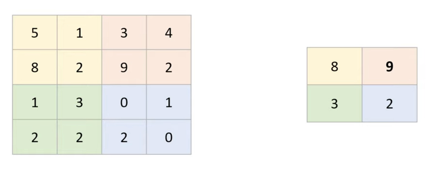
After each convolutional layer, there is a pooling layer. Pooling Layers are used to downsample the feature map, keeping the most important parts and discarding the rest. A 2x2 filter is applied across the feature map, and the largest pixel value in each region is saved to the new output feature map. Max Pooling is important, because it reduces the dimensions and consequently the amount of computation. It also makes the model tolerant to distortion and variations because we’re just capturing the main feature.
After the final pooling layer, the 3d Feature Maps for the higher level features like head and body are flattened together into a comprehensive 2d array. This is then fed into the Fully-Connected(FC) Neural Network layer for classification. The FC layer in CNNs takes the features extracted by the convolutional layers and uses them to make final predictions. It connects every neuron from the previous layer to every neuron in the next, acting like a traditional neural network layer. This layer helps in combining the features to classify the image into specific categories. In this case Koala or not Koala!

Important Note(ReLU):

After every convolution layer, and before max pooling, the ReLU function is applied to the feature maps. All ReLU does is convert any negative input to 0, keeping positive inputs the same. ReLU introduces non-linearity to the model by transforming the input, allowing the model to capture more complex relationships in the data.
The Beauty of ConvNets:
At this point you might be wondering, how does the computer know what filters correspond to an ear or an eye? And, that’s what makes CNNs so amazing. When training a Convolutional Neural Network, it will automatically learn to detect relevant features because you are supplying thousands of Koala images. Initially, filters in the convolutional layers are assigned random values. The network makes predictions based on the current state of the filters, which are compared to the actual labels using a loss function. Backpropagation then adjusts the filter values by computing gradients and updating the weights to minimize the loss. This process is repeated over thousands of images and multiple epochs, gradually refining the filters to detect increasingly complex and relevant features, such as edges, textures, and eventually parts of objects, leading to accurate image classification.
Applications In Identifying Brain Tumors:
Applying this concept to the human brain, leads to incredible insights into the nature of classifying brain tumors. CNNs can detect subtle and complex patterns in the image data that may be too intricate for physicians to notice. As CNNs progress through layers, they learn increasingly abstract features. Early layers may detect edges and textures, while deeper layers can combine these into more complex shapes and structures, potentially identifying patterns not immediately obvious to human observers. Brain Tumors have complex and varied appearances that go beyond simple visual patterns. CNNs can learn to recognize these complex patterns and structures through deep layers, providing new insights and accuracy to the field of radiology.
A 2023 study introduced BCM-CNN, a Deep Learning model that classified brain tumors as malignant or benign based on fMRI images with 99.98% accuracy. The CNN model was pre-trained with thousands of medical images, particularly for the classification of brain tumors(Gamel et. al, 2023)

A 2019 study proposed a CNN technique for a three-class classification to distinguish between three kinds of brain tumors, including glioma, meningioma, and pituitary tumors. They used a pre-trained GoogleNet for feature extraction from brain MRI scans. The system recorded a classification accuracy of 98.1%, outperforming all state-of-the-art methods(Deepak et. al, 2019).

Brain tumors are ranked 10th among major causes of death in the US with about 17,200 people dying annually. The old method of manually evaluating medical imaging is time-consuming, inaccurate, and prone to human error. While doctors will always be a valuable part of critical care, assistance from AI technologies can greatly improve our understanding of patient conditions and hopefully save many lives.
Sources: These are great resources, definitely check them out!